INTRODUCTION
Calculating the parameters of a high vacuum system can be a tedious and daunting task, involving a significant amount of factors, as well as good estimates and approximations for a variety of parameters. Because a vacuum system involves highly dynamic and complex processes, as well as having significant variability in performance based on environmental conditions, processes, system conditioning, operating procedures, virtual leaks, real leaks, and a wide range of other problems one might encounter operating such a system, approximations of system performance are at best rough indicators to what to expect. In addition, not all data is published or explicitly defined for certain system parameters, requiring best guess approximations. However, one can both calculate and simulate system performance to a good degree of accuracy to establish what might be expected during ideal, nominal conditions. This blog post will walk through a simple process for estimating some of the pumping parameters for a system utilizing an oil diffusion pump, which will be further used for estimating system performance and running molecular flow models for the Integrated High Vacuum Test Stand pumping assembly.
PROBLEM OVERVIEW
In order to estimate expected system performance of the pumping assembly in the Integrated High Vacuum Test Stand, numerous calculations need to be made to gauge the key characteristics of the system. This includes conductance, effective speed of the system, ultimate blank-off pressure, and performance under various gas loads. All of the hand calculations for the system can be found on the Integrated High Vacuum Test Stand page for reference. Other past blog entries have detailed the process in calculating these basic parameters (see the table of contents page for the High Vacuum Calculation Walkthrough series.) To summarize very briefly on the subject, there are three major parameters used in the calculation of high vacuum systems: speed, pressure, and gas load. This is defined by the fundamental governing equation S=Q/P, where S is the speed of the system, Q is the total system gas load, and P is the pressure. While an incredibly simple and powerful formula, the challenge lies in calculating the total amounts for each of these parameters and accounting for all variables in the system.
To find S, we must determine conductance of the system. While all vacuum pumps are rated for a particular speed (for a given gas at a given temperature), unless the pump inlet is connected directly to the chamber, the speed seen at the chamber will not be the same seen at the pump inlet. This is due to conductance of the components between the pump and the chamber. Almost always, there is some sort of adapter plates, baffles, traps, pumping lines, and/or isolating valves between a pump inlet and the chamber inlet. As a result, the effective speed must be calculated for the system and used for estimating pumping conditions of the system for a given chamber.
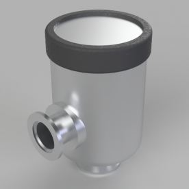
The starting place here will first be to look at the pump datasheet. All pumps will be rated for some speed with a certain gas, and almost always quoted for air at 20C, which is a standard for vacuum pumping specifications. For the pump used in the system, the Edwards EO4 diffusion pump, the speed is rated at 600 L/s for air. Additional resources also show that it is rated for 800 L/s for hydrogen. A key thing to remember for calculating system parameters for high vacuum conditions in molecular flow is that conditions must be calculated separately for each gas in the system. Air is a good approximation, however pumping speed varies for atomic mass as well as temperature, and depending on the process and the system, the pumping speed can be radically different.
Conductance is then calculated for the entire pumping system. This is found by combining the conductances of each individual component in the system to find the total effective conductance, and using this to calculate the effective speed with the actual pump speed as described above. Full calculations for the system are found in the above project page for reference. Once conductance is calculated, effective speed can be found with the equation:
S(eff)=[S(pump)xC(total)]/[S(pump)+C(total)]
Again, note that this must be calculated for each gas used. Air is the easiest, since numbers and pumping curves are generally present in the datasheet. Hydrogen in this case is also possible since pumping speed for molecular flow is generally given for this gas as well. But what happens when you need to calculate any other gas or element? To calculate this all out by hand would be immensely time consuming and tedious for every element, and is not practical. However, we can estimate the resulting pump speed vs atomic mass with a simple approximation.
APPROXIMATING PUMP SPEED FOR AN UNKNOWN AMU
In order to estimate the system performance for any gas, we need to first figure out effective speeds. Note that in the equation above, effective speed requires actual speed of the pump at the inlet. One way to approximate this is simple to use the value for air for other gases. However, this will increase the error and reduce the accuracy of your predictions. Looking at pumping and performance characteristics for gases and molecular flow, you will find that this is a nonlinear relationship. Different pumps will also have different response curves at different vacuum levels for different gases. So a turbopump response will be very different from an ion pump response, which will be very different from a diffusion pump response. In each of these categories, response can vary between the same style of pump. There are numerous types of ion pumps, usually optimized for a particular set of gases. For the diffusion pump, a simple curve of best fit was used between the two known pumping speeds of hydrogen and air. Knowing that speed is nonlinear for different gases, the curve of fit selected was a decaying exponential. This can be observed through the general conductance equations for molecular flow, giving a more reasonable (although still not 100% accurate estimate) for gases. For the diffusion pump used, the resulting curve and fit equation is as follows:
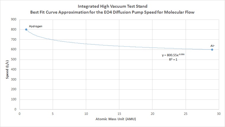
Using the derived equation from the line of best fit between the two known values of hydrogen and air for the pump, we can calculate the estimated derived speeds for any other atomic mass. Plotting the new curve for every atomic mass unit in the periodic table, we get the following curve:
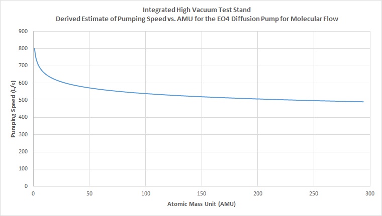
With this curve, we now have a better estimate for pumping speed of the diffusion pump for any atomic mass. Using these approximations, we can now go back to our original equations for calculating effective speed, and solve for the effective speed of the system for a particular gas by using the approximated pump of the speed as well as hard calculated numbers for effective conductance of the high vacuum pipeline and connecting components for the given gas.
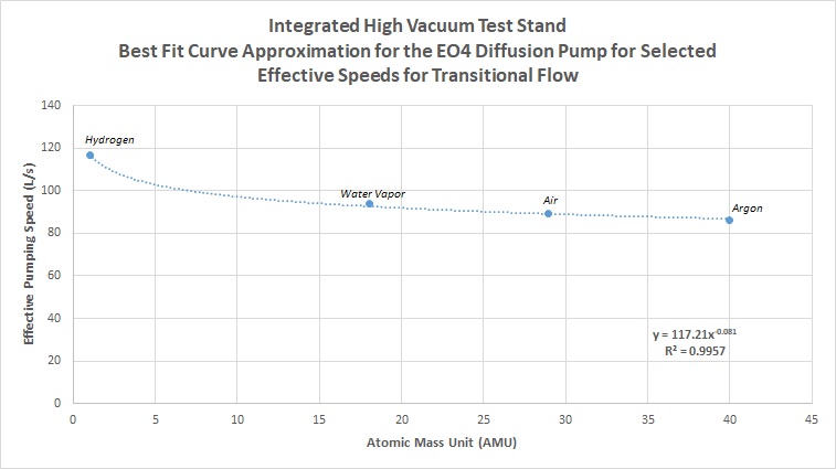
We can also approximate pumping speed for the pump in transitional flow in the same way. This however requires a few extra steps. Normally in diffusion pump data sheets, the pumping speed vs. pressure curve is given, typically for air. The above data was derived for molecular flow, or high vacuum conditions generally at and lower than 10^-4 torr. For the region between 10^-1 to 10^-3 torr, transitional flow occurs. We can get an estimated number by tracing along the curve to find the speed for a given pressure. In this case, transitional flow numbers were estimated for a pressure of 10^-2 torr. Tracing the speed vs pressure curve in the data sheet, a speed of 100 L/s can be seen for around 10^-2 torr. To get our line of best fit approximation, we still need one more value. While values are not generally plotted for other gases, we do know that usually values for both air and hydrogen are given for molecular flow. Looking across numerous datasheets for various diffusion pumps, we can see that in general the speed for hydrogen is about 25% higher than that for air. In this case, for transitional flow, we estimate the speed for hydrogen to be 125 L/s, based off of a 25% increase in speed from 100 L/s for air. Following the same steps as above, we first graph the estimated best fit curve between air and hydrogen for transitional flow:
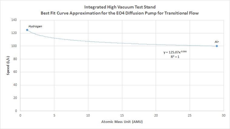
Then we use this equation to derive an estimate for all other atomic masses:
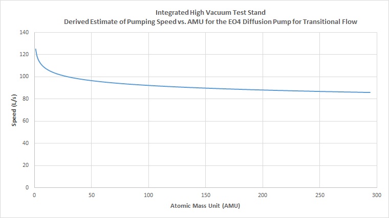
With these numbers established, we can move on to the next step of approximating the effective system speed using these derived numbers.
APPROXIMATING EFFECTIVE SYSTEM SPEED USING DERIVED PUMPING SPEED RESULTS
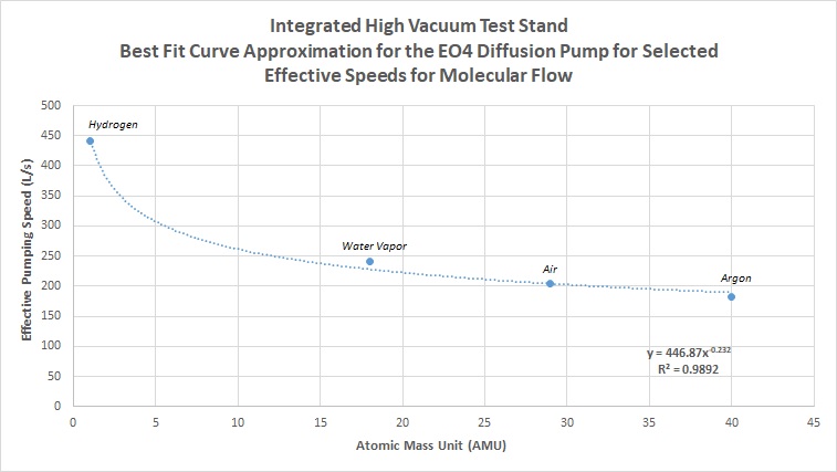
With the pump speeds estimated for any atomic mass, effective speed of the system can now be calculated, and a similar curve derived. For this step, it is recommended to calculate the effective speed of the system for numerous gases to produce a more accurate best fit curve for approximating all other atomic masses. This means using the actual equations and correction factors for conductance and effective speed for the selected gases. For the above system, common gases were selected for actual calculated estimates, which include air, hydrogen, argon, and water vapor. Water vapor in particular becomes useful when estimating the ultimate pressure of a system during pumpdown in molecular flow, since at high vacuum levels water vapor becomes the dominant gas load for a system due to outgassing, until ultra-high vacuum levels are reached (past 10^-8 Torr), where hydrogen becomes the dominant outgassing load. Going through the entire calculation process, the following numbers were calculated for the four gases:
- Air = 204 L/s
- Hydrogen = 441 L/s
- Argon = 182 L/s
- Water Vapor = 241 L/s
These above numbers are plotted, and a line of best fit is established:
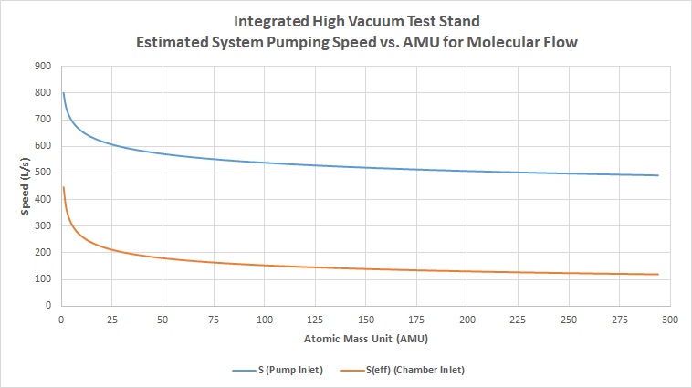
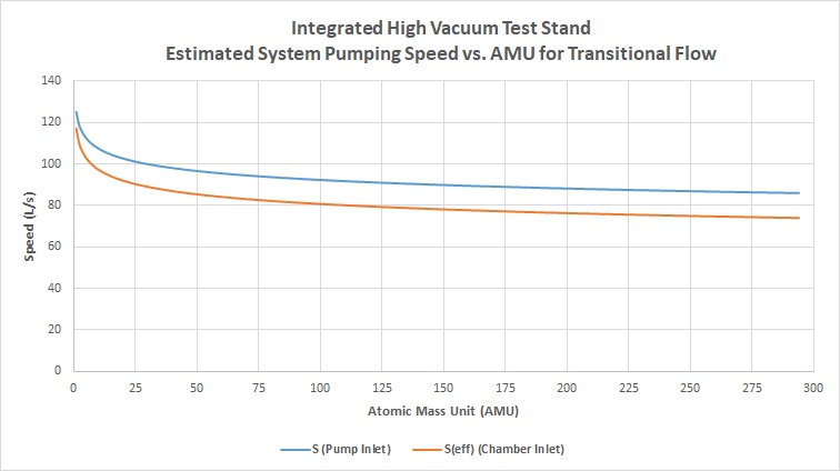
Between hard calculated numbers and the actual curve fit, values can range +/-10%, however this still gives us a very reasonable guess to system performance based on extremely little starting data. Using the above derived equation, we can do the same as in the prior section, and calculate estimated values of pumping speed for all atomic masses. In this graph, the speed of the pump and the effective speed of the system at the inlet of the chamber are directly compared:
And again, we calculate the actual numbers for transitional flow for air, hydrogen, argon, and water vapor, getting the following data and plotting for a line of best fit:
- Air = 89 L/s
- Hydrogen = 117 L/s
- Argon = 86 L/s
- Water Vapor = 94 L/s
And the resulting graph comparing the effective speed at the inlet of the chamber to the effective speed at the inlet of the baffle for transitional flow:
CONCLUSION
Using the above method for deriving estimates of various speeds using information from datasheets, literature, and principles of high vacuum engineering, we can simplify the process to estimate pumping speeds for any atomic mass in a diffusion pump based system. This method can be applied to any high vacuum pumping setup, as long as the appropriate values, responses, and curves are used for the selected pump. By calculating a few basic and common gases, values can be derived for other elements. This is especially important for high vacuum applications, where molecular and transitional flow estimates must be made separately for each gas species present in the system. The estimated values and curves are by no means exact numbers, but should serve as rough guidelines for what to expect for a given system response.