COMPARISON BETWEEN SYSTEM V2 CALCULATIONS AND ESTIMATES USING DUSHMANS TABLE
In the previous Chapter 3.1, we explored the calculations for system conductance and effective speed in molecular flow for the V2 design iteration. This was calculated using a rather long and tedious method involving finding the conductances for every individual part. Let us compare this to a simpler estimate to better understand the results, and assume that we are to calculate the conductance of System V2 using a very simplified estimate from Dushmans Table. This can also help illustrate when simplified calculations vs. more intensive calculations may be used for determining molecular flow estimates based on system complexity.
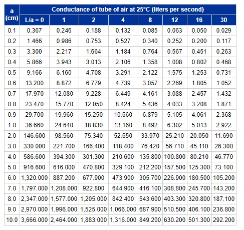
Dushmans Table is an empirically derived method for approximating conductances of tubes. Using this approach, we would assume the entire pipeline with all its elements are a single element of equivalent length with constant diameter. An example reference to this table can be seen here:
Conductance Calculations Using Dushmans Table
The table from the above source from the KJL website is pulled and shown below (credit for the table is attributed to Kurt J. Lesker):
From System V2 measurements, we know the following parameters:
Total Effective Length = 26.244cm
Average Diameter of 2.75” CF Hardware = 3.556cm
The radius is then 1.778cm. Dividing the length by the radius gives the “L/a” ratio of 14.760, where “L” is length and “a” is radius. Following the table down the “a” column, we end up between rows 1.0 and 2.0. Following this over to the L/a ratio column, we lie somewhere between 12 and 16. This roughly approximates to a conductance value between the lower and upper bounds of 5.013 and 25.210. If we interpolate this data between these major bounds, we can generate a table such as the one below:
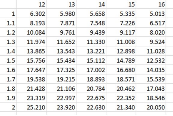
We can now see that we get a closer approximation of the conductance between the bounds of 1.7 to 1.8 and 14 to 15, of a conductance between 18.571 and 20.784. This conductance is higher than those for air, argon, and water vapor, but less than that of deuterium – in fact, it is almost exactly in the middle of the two extremes between argon and deuterium. This shows that we are well within the expected ballpark for our original intensive calculations. The above method using Dushmans Table however does not account for temperature, molecular mass, or other correction factors for short pipes. Also note that this estimate was found using a straight length of pipe equivalent to length of the actual system, with no bends. If we included the bends in our estimation using the table method, this number would be much lower, and hence much closer to the values similar to air. Thus we can show within reasonable agreement and certainty that breaking down each individual component of a pipeline, applying correction factors, and summing the total for series conductance, is within the expected range, even when compared with very simplified methods of estimation.
While using Dushmans Table and extrapolating results in a good first estimate, it is still a very rough number and should only be used to get a very rough ballpark estimate. For more complex components besides straight pipes, full calculation should be employed to get a more accurate system estimate, and it is recommended to go through the more rigorous calculations to get better estimates of how a system would behave, especially if different gases, temperatures, and multiple components are being considered.