CALCULATIONS FOR CONDUCTANCES AND EFFECTIVE SPEEDS IN MOLECULAR FLOW FOR VARIOUS PROCESS GASES
SYSTEM DESIGN V2
SECTION 1 – Design Overview
Based on the prior mentioned availability of a 2.75” CF inline valve, a decision was made to redesign V1. Up until this point no calculations were made influencing design decisions, which were based on general knowledge of vacuum systems, since system V1 was the first design concept based on the most immediately available components. Subsequent design iterations however were directly influenced by the calculation results from the molecular flow numbers derived from the system. Below is a rendering of the V2 design:
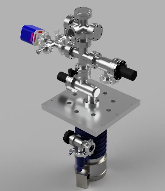
The new inline valve would allow for a more direct pumping path, and have a vertical topology. The main crosses were kept and just re-oriented to save functionality of the previous system. The third port on the KF25 cross was also decided to be dedicated for gas input and venting the system to atmosphere, and the remaining KF25 inputs stayed the same (thermocouple gauge and high vacuum gauge.) One downside to the valve however was that it was pneumatic – while cheap, it means that there is no control over the effective speed of the system if needed, for example, for a fusor. This required the additional use of some sort of manual valve. After weeks of searching, a 2.75” Conflat manual butterfly valve was located on eBay. This valve also had an additional bonus of being both a sealing and conductance throttle valve, and was found at a very low price. The overall cost slightly increased from V1, however it made for a more convenient chamber to mount and work with physically, while allowing for better flow control and potentially better conductance along a more direct path to the chamber.
In order to further understand how system topology would affect high vacuum pumping behavior, calculations on this design were performed to determine its viability before too many parts were purchased. Unfortunately some valves and parts were already bought due to the fast nature of things popping up and disappearing on eBay – some of which ended up being recycled to new designs, others are still unused due to further design changes. From V1 to V2 however, this design satisfies more of the initial requirements stated in the Introduction and Chapter 2 of this series. Form factor, functionality, and control was gained, however at slightly higher cost. Conductances and speeds, as illustrated below, did not seem to be as good as initially hoped however.
SECTION 2 – Calculations for Determining Conductance and Effective Speed in Molecular Flow
Below are the PDFs with the calculations performed on the V2 design to determine conductance and effective pumping speeds in molecular flow for the following gases: air, argon, deuterium, and water vapor:
2.75″ Conflat High Vacuum System – Design Iteration 2 – Molecular Flow – AIR
2.75″ Conflat High Vacuum System – Design Iteration 2 – Molecular Flow – ARGON
2.75″ Conflat High Vacuum System – Design Iteration 2 – Molecular Flow – DEUTERIUM
2.75″ Conflat High Vacuum System – Design Iteration 2 – Molecular Flow – WATER VAPOR
In order to determine the effective speed of the system, both conductance and maximum pumping speed of the high vacuum pump are needed, given the gas load Q and the ultimate pressure P of the system are unknown. The equations and all of the definitions are in the PDFs for reference. As an important note going forward, effective speed is not the same as the speed of the pump. Effective speed is the total speed of the system accounting for the speed of the pump and the conductances of the pipeline to the chamber. Effective speed is practically always lower than the pump speed, never higher. The key limiting factor of conductance in a system is dictated by the component with the lowest conductance – that component represents a choke point in the conductance where the total conductance and effective pumping speed will be lower than the conductance of that component. Thus for a system based off of 2.75” CF hardware, you are always limited to the theoretical max limit of conductance for that size pipe, regardless of pump speed. Conductance drastically falls off for length, and for short pipes conductance may be less than initially anticipated due to correction factors required when calculating the numbers for such pipes and components.
The max speed of the pump to be used in the system is already known, at 600 L/s for air and 800 L/s for hydrogen, based off the datasheet (the pump is an Edwards EO4 diff pump.) This is represented in Section 1 of the above PDFs.
For calculating the conductance of the pipeline, one approach would be to find the equivalent conductance of a length of pipe for all the parts, assuming the internal diameter stays the same. However, a more accurate approach for finding the worst case conductance under ideal conditions would be to find the conductance of each individual component in the pipeline, and sum all of the conductances – note that series conductances for vacuum systems, when summed, are calculated like resistors in parallel. By finding the total conductance from all the sums, correction factors can be applied for each component, giving a worst-case scenario conductance for the system. In reality, the conductance may probably be higher since everything calculated in the above PDFs are using the largest correction factor numbers for the appropriate calculations as experimentally determined in literature on the subject.
The conductances are calculated in order of the component, from diffusion pump up to the chamber, which is the 5 way cross. Note that each part is calculated in multiple stages. First, the conductance is found using the general formula for a tube. However, since the L/D ratio for the components is less than 5, corrections must be applied. Next, the equation for short pipes is calculated using the number for a long pipe. Then, a further error factor correction of about 12% max is factored in to the number, resulting in the final conductance for that part. This 12% is a correction factored applied based on experimental data observed in literature for air @20C, which provides the maximum deviation for the given L/D ratio. Other gases are approximated and estimated to give rough numbers using this correction factor as well for simplicity.
Note that the choke point in the system is actually the inline valve, calculated in Section 3. Even though the valve is technically “linear” in fashion, it actually is not a full straight-through gate valve, and hence must be approximated with x2 90 degree bends in series, which cuts the original conductance of the valve in half. This is the limiting factor of the system. Inline valves such as this generally have lower conductance than an equivalent 90 degree valve, despite the fact it looks like the flow is straight through. One should note that motion in molecular flow is random, which plays a large factor in the behavior of gas flow in high vacuum systems, and does not behave as initially expected under non-molecular flows.
In Section 4, the butterfly valve is calculated, and the valve portion must be accounted for in the area of the opening. Even in the fully open position, it still adds impedance. The ratio of the equivalent area was found to be 65.8%, which was applied as an additional correction factor to the valve conductance.
The following sums up the total system conductance and effective pumping speed of the system in molecular flow for each of the gases, calculated in Section 6 of the PDFs:
AIR:
- Conductance – 8.737 L/s
- Effective Speed – 8.612 L/s
ARGON:
- Conductance – 7.440 L/s
- Effective Speed – 7.349 L/s
DEUTERIUM:
- Conductance – 33.137 L/s
- Effective Speed – 31.819 L/s
WATER VAPOR:
- Conductance – 11.078 L/s
- Effective Speed – 10.877 L/s
As can be seen from the above numbers, the conductances and speeds of the system, despite having a very short and direct pipeline, are surprisingly small, except for deuterium. As expected, with all things equal, it can be seen that molecular weight has a direct result on the conductance of a system in molecular flow. The pump, starting with a speed of 600 L/s, has been effectively reduced by more than an order of magnitude, to around 10 L/s for the various process gases (much higher for deuterium). Although these numbers may be ok for deuterium, extra room was desired for argon, in addition to being able to handle more loading from water vapor. Because of this, a new topology was designed and calculated in the same manner to compare numbers to see if these estimates could be improved. This will be seen in the next chapter covering the design V3 for molecular flow. However, the actual gas handling load due to effective speed will not be known until after ultimate pumpdown pressure is calculated due to water vapor loading, and applying this number for gases involved at all pressures that will be experimented at.
As a final side note on this section and going forward, the calculations were started for molecular flow since this is the very first step for figuring out the system when gas loads and ultimate pressure are unknown. These will be derived in later sections from these results. Also note that the low vacuum, roughing portion is not covered until later. This is due to the fact that the roughing pump parameters are not needed for these high vacuum calculations, and it is in the high vacuum regime that the system will be primarily operating in. For the time being, the only parameter really required for the roughing pump is to make sure that it meets the backing requirements of the diffusion pump. This will be covered in later chapters dealing with the roughing pump criteria.